Demand Simulations under Weather Uncertainty
Overview
Gas Demand Simulation is an analytical process that leverages simulations and ML techniques to predict total gas demand in a specific country for a given weather scenario. In fact, multiple weather scenarios are fed into the simulation process to generate a range of possible demand outcomes. At the minute, included countries are: GB, DE, FR, NL, BE, IT, ES, DK, PL, AT
The logical framework of the Demand Simulator is depicted in the following diagram:

Blocks Details and related AML Pipelines
Let's dive into the details of the Demand Simulations describing block by block:
- Block A: in this block of steps Demand models per country are trained considering historical data, actual weather data and calendar features. Breaking down the steps:
- The FSM training dataset creation, which currently involves the skeleton, historical data and calendar features, is enriched with weather actual data (max temperature, min temperature, cloud cover, wind speed).
The related pipeline is the following:
 So a one-step pipeline is executed to prepare the dataset for training the demand models.
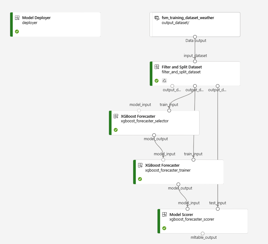
- Models are then trained using a ML class (specifically, an XGBoost). The XGBoost class leverages the current mlflow + sktime type of model developed for the base stack of the FSM. The model that is adopted at this stage is configurable and can be easily replaced with a different model. At the end of this block, models are registered in the AML model registry.
The related pipeline is the same of a standard FSM model training pipeline, with just XGBoost as a model type. The pipeline is depicted below:
So a one-step pipeline is executed to prepare the dataset for training the demand models.
- Models are then trained using a ML class (specifically, an XGBoost). The XGBoost class leverages the current mlflow + sktime type of model developed for the base stack of the FSM. The model that is adopted at this stage is configurable and can be easily replaced with a different model. At the end of this block, models are registered in the AML model registry.
The related pipeline is the same of a standard FSM model training pipeline, with just XGBoost as a model type. The pipeline is depicted below:
-
Block B: in this block of steps, weather scenarios are generated.
- In the first step, a distribution fitting is performed on the historical weather data to generate a distribution of weather features. Essentially, this is done by training a Bayesian Gaussian Mixture (BGM) model on the historical weather data, considering the raw weather features as input (max temperature, min temperature, cloud cover, wind speed). Once models are trained, they are registered in the AML model registry.
The related pipeline is the following:

Since the pipeline doesn't involve the creation of a test set (to train a generative model a test set is not mandatory), the third execution of the bgm_sampler_training (namely,
bgm_sampler_trainer), repeats the training process but labelling it with a "testing" tag, in order to accomplish with the deployer component requirements.- In the second step, the weather scenarios are simulated adopting a Monte Carlo approach. The weather features are sampled from the BGM sampler models generated in the previous step until stability is reached over a single year (that means that depending on the randomness of a simulation, different simulated years can have a different number of simulations). The weather scenarios are then saved into the Data Lake.
The related pipeline is the depicted below:

-
Block C: Block C steps put together what happens in Block A and B:
- The first step is a twofold data preparation task:
- Firstly, the FSM prediction dataset is enriched with the weather actual data. The same pipeline running in Block A is executed to prepare the dataset for prediction, but configured for having a prediction dataset that covers the entirety of the forecast horizon.
- Secondly, the dataset is filtered by country and total demand as asset type, and the weather scenarios generated in Block B are then appended to the dataset. In doing so, in order to have the same nr of run across each year, the minimum of the number of runs per year is considered (e.g. for country GB, if 2025 has 500 runs and 2026 has 400, 400 is then considered for both years).
The reason why we filter by country and total demand is to avoid an exploding join operation: the primary key of weather scenarios is the combination of country, date, run_nr and batch_nr, while on the other side, the primary key of the prediction dataset is composed by the following columns:
- "asset_name",
- "asset_type",
- "asset_id",
- "source",
- "units",
- "level",
- "variable",
- "country_to",
- "country_from",
- "country_code",
- Demand is predicted using the models trained in Block A and the weather scenarios generated in Block B. These simulations are saved into the Data Lake. This jobs execute a sweep job execution over the different runs of the weather scenarios. SO the sweep job will create a child job for each run of the weather scenarios. At the moment, the sweep executes up to 100 runs in parallel.
The second element of the aforementioned data preparation task is joint with the demand prediction task in the following pipeline, per country involved:

Please do ignore the skeleton prediction data and the historical daily ones, they are just placeholders for making the dataset_builder component running smoothly.
- On top of that, this dataset will be used to draw percentiles or upper/lower bound interval for gas demand in a given country. The way percentiles or bounds will be calculated is still to be refined according to traders' requirements.
- The first step is a twofold data preparation task:
Orchestration
Demand simulations run on demand, with a low frequency (2-3 times a year, especially ahead of the winter period). The blocks reported in the overview section are orchestrated by AML jobs. To manually run it, it is necessary to to run the script runner.py with the different parameters configuration from the config_latest.toml file:
- execute training of the BGM weather samplers (distribution fitting):
- models_scope should contain "weather_sampler" as a value
- weather_sampler_training_also = true
- weather_sampler_training_type = "full"
- submit_weather_sampler_training = true
- execute simulation of the weather scenarios:
- models_scope should contain "weather_simulator" as a value
- weather_simulator_also = true
- submit_weather_simulator = true
- execute training of the demand models:
- models_scope should contain "demand_model_weather" as a value
- demand_model_weather_training_also = true
- submit_training = true
- execute demand simulations:
- models_scope should contain "demand_model_weather" as a value
- demand_model_weather_simulation_also = true
- submit_prediction = true
- update the training/prediction dataset:
- models_scope should contain "demand_model_weather" as a value
- dataprep_demand_weather_also = true
- submit_dataprep = true
To modify any key parameters of the Demand Simulations components execution please refer to the following sections of the config_latest.toml:
- [dataprep_demand_weather_simulation.training]
- [dataprep_demand_weather_simulation.prediction]
- [weather_country_list]
- [weather_month_list]
Environment
For the execution of steps included in block A and C, the environment is the same used by the ML models part of the base stack of the FSM, namely the ML-forecasting-models-env:<latest_version>.
For the execution of block B, files for environment definition and registration can be found at the path weather-simulator/manifests/ of the ngtt-fsm repo. Currently, the environment has to be registered in AML.
Component & Modelling
Some components were specifically developed for the Demand Simulations, while others are shared with the base stack of the FSM.
The brand new components developed are:
- bgm_sampler: this component is responsible for the training of the BGM models used to generate weather scenarios. Per each country and month of the year, a dedicated BGM model is trained. The key parameter of a standard Gaussian Mixture model is n_components,that defines the number of components in the mixture model. The Bayesian version differs to the standard one since n_components is considered as a sort of upper bound, and a likelihood to each component is assigned (which means that low likelihood components are less relevant in generating new data). More details can be found presentation and at this paper.
- weather_simulator: this component is responsible for the simulation of the weather scenarios. As mentioned above, the approach is based on Monte Carlo simulations, where the samples are drawn from the BGM models trained.
Components shared with the base stack of the FSM and that were adjusted to accomplish some specificities of the processes involved are: - dataset_builder - scoring
The components are registered/updated in AML automatically by the Build & Deploy GHA. Files for component definition can be found within the ngtt-fsm repo.
Manual evaluation of model performance
The Demand Simulation process is used as a forecasting model that supports boundaries definion for expected demand level,
For the forecasting model, when choosing the optimal parameter of the XGBoost Forecaster (e.g. features, nr of estimators, ...), backtesting experiments have been executed to quantitatively evaluate the performances of the model adopting weather data, with the same logic adopted in the foundation modelling stack of the FSM.
Rergarding the weather sampler, a different approach has been adopted.
First, a quantitative metric namely the energy_ratio has been adopted, to identify the most promising BGM models. Then, within the top 3 candidates per each model (country-month), we selected the one with the lowest number of components, to avoid overfitting.
The energy ratio is founded on the concept of energy distance, a metric that measures the distance between two distributions X and Y. The energy distance is defined as follows:
$$
D(X, Y) = 2E||X - Y|| - E||X - X'|| - E||Y - Y'||
$$
MOre details in the paper that introduced the concept of energy distance for statistical samples.
Forecasting Model metric score(s)
Below we reports the main metrics that have been used to evaluate the forecasting models.
2021 and 2022 years were used as test sets.
| Metric | Full metric name | Expression | Comments |
|---|---|---|---|
| MAE | Mean Average Error | \(\frac{1}{n}\sum_{i=1}^n\left\|y_i-\hat{y}_i\right\|\) | Easily interpretable, but does not reveal the proportional scale of the error |
| MAPE | Mean Average Percentage Error | \(\frac{100}{n} \sum_{i=1}^n\left\|\frac{y_t-\hat{y}_i}{y_i}\right\|\) | Ideal when comparing performance between different data sets, but values might explode if test set contains values close to zero. |
Weather Sampler metric score(s)
Below we reports the main metrics that have been used to evaluate the weather sampler models.
| Metric | Full metric name | Expression | Comments |
|---|---|---|---|
| Energy Ratio | Energy Ratio | \(\frac{p-value}{D(X, Y)}\) | The ratio between the p-value of the energy distance and the energy distance itself. The lower the distance or the higher the p-value (or both factors combined), the better the distribution fitting model |
Future Developments and Suggested Improvements
Here below a list of what we suggest to be the next steps for the demand simulations based on weather uncertainty: - switch to a non recursive approach for demand predictions, in order to speed up the process. One option could be to train the model using only calendar features and weather features. Another option could be to adopt a direct strategy, so training a specific model for target horizon - Adopt a time-dependent approach to generate weather scenarios. At the moment, individual days are sampled independently. - re-use the under-development new demand models to generate the predictions